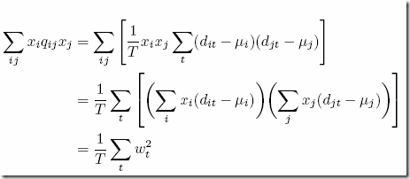
Here is an interesting but obscure reformulation that sometimes performs better than the traditional x’Qx term in a mean-variance portfolio model. We notice that the covariances can be calculated as:
 where μi is the mean return and di,t are the historical data. We now can write:
This is especially a good formulation if there are more instruments than time periods (in large practical problems this is often the case as older historical data is not considered as having much predictive value). The corresponding OML model, where we solve K sub-problems at the same time, can look like (see post for more info):
Model[
Parameters[Sets,I,K,T],
Parameters[Integers,Selected[I]],
Parameters[Reals,Return[I]],
Parameters[Reals,Lambda[K]],
Parameters[Reals,MeanAdjRet[I,T]],
Parameters[Integers,TT[]],Decisions[Reals[0,Infinity],Alloc[K,I]],
Decisions[Reals,w[K,T]],Constraints[
Foreach[{k,K},FilteredSum[{i,I},Selected[i]>0,Alloc[k,i]]==1],
Foreach[{k,K},{t,T},w[k,t]==FilteredSum[{i,I},Selected[i]>0,MeanAdjRet[i,t]*Alloc[k,i]]]
],Goals[Minimize["Overall"->
Sum[{k,K},
Sum[{t,T},w[k,t]^2]/TT[]
- Lambda[k]*FilteredSum[{i,I},Selected[i]>0,Return[i]*Alloc[k,i]]
]
]]
]
As an aside: this formulation also shows how this can be linearized: replace ∑w2 by ∑|w|.


No comments:
Post a Comment